Overview:

In this short article, I am going to show how sentence transformers can be used to create embeddings of text and how to use DBSCAN to detect clusters.

Install Dependencies:

Install the below dependencies,

!pip install -U sentence-transformers
!pip install sklearn
!pip install plotly
!pip install nbformat>=4.2.0
!pip install matplotlib

Import Dependencies:

import pandas as pd
import numpy as np
import plotly.graph_objects as go
import pickle
import matplotlib.pyplot as plt
from sentence_transformers import SentenceTransformer, util
from sklearn.neighbors import NearestNeighbors
from sklearn.cluster import DBSCAN

Data Cleaning:

I was using some custom data which had many inconsistencies. You can create your script for data cleaning. Mine is as below,

def data_cleaning(input_file, output_file):
    list_data = ["<br/>","Hi team -","hi team -","Hello-","Hi Team,","Hi team,","Hello,","Hi Team:","Hello Team,","Hi,","Hi team-",
                 "Hi Team-","Hi Team.","Hello,","hello,","Hi Team","hi team","hello team","Hello!","team,","Team","====","HI","Hi team"]

    with open(input_file, 'r') as file:
        data = file.read()
        for l_data in list_data:
            data = data.replace(l_data, "")

    # Opening our text file in write only mode to write the replaced content
    with open(output_file, 'w') as file:
        file.write(data)

    df = pd.read_csv(output_file)
    # Renaming the column
    df.rename(columns={"First Comment": "comments"}, inplace=True)
    # Removing blank rows
    df.dropna(inplace=True)
    df.reset_index(drop=True, inplace=True)
    df.to_csv(output_file, index=False)
    number_of_rows_input_file = pd.read_csv(input_file).shape[0]
    number_of_rows_output_file = pd.read_csv(output_file).shape[0]
    print(f"Number of rows in {input_file} = {number_of_rows_input_file}\n" +
          f"Number of rows in {output_file} = {number_of_rows_output_file}\n" +
          f"Number of rows dropped = {number_of_rows_input_file - number_of_rows_output_file}\n")
    print(f"Data cleaning complete. Cleaned data is stored in {output_file}")

# Call the function
data_cleaning("./Data/Raw_Dataset.csv", "./Data/Cleaned_Dataset.csv")

Convert the cleaned dataset to a list:

We need to convert the cleaned dataset to a list to use in sentence transformers for creating embeddings.

# Converting the cleaned dataset into list

df1 = pd.read_csv("./Data/Cleaned_Dataset.csv")
comments_list = df1.comments.tolist()

Model to create embeddings:

We are using sentence transformers to create embeddings.

• You can use any model that is supported by sentence transformers. I am using all-MiniLM-L6-v2.

• distilbert-base-nli-stsb-quora-ranking is also another good alternative.

def create_and_store_embeddings() -> np.ndarray:
    model = SentenceTransformer('all-MiniLM-L6-v2')
    embeddings = model.encode(comments_list, show_progress_bar=True)
    # Normalize the embeddings to unit length
    embeddings = embeddings /  np.linalg.norm(embeddings, axis=1, keepdims=True)
    return embeddings

# Call the function
create_and_store_embeddings()

Storing the embeddings:

Store the embeddings so that we don't have to create them every time.

# Store sentences and embeddings to disc
with open("./Data/embeddings.pkl", "wb") as fOut:
    pickle.dump({'sentences': comments_list, 'embeddings': embeddings}, fOut, protocol=pickle.HIGHEST_PROTOCOL)

Loading the stored embeddings:

Load the embeddings from the already created pickle file as below,

#Load sentences & embeddings from disc
embeddings = np.empty_like(embeddings)
with open("./Data/embeddings.pkl", "rb") as fIn:
    stored_data = pickle.load(fIn)
    stored_sentences = stored_data['sentences']
    embeddings = stored_data['embeddings']

Detect Clusters:

Elbow Method:

To detect the clusters using DBSCAN, we need to find the eps value.

This value can be found by using the Elbow Method. The flow of the method is defined below,

• Compute the k-distance graph: Calculate the distance between each point and its kth nearest neighbor (e.g., k=4).

• Sort the distances in ascending order and plot them.

• Look for the "elbow point" in the plot, which is the point where the curve starts to bend or the rate of change in distances decreases significantly.

• Use the distance value at the elbow point as the eps value for DBSCAN.

def find_optimal_eps(embeddings, k=4):
    neighbors = NearestNeighbors(n_neighbors=k+1, metric='cosine')
    neighbors_fit = neighbors.fit(embeddings)
    distances, _ = neighbors_fit.kneighbors(embeddings)
    sorted_distances = np.sort(distances[:, -1], axis=0)

    plt.plot(sorted_distances)
    plt.xlabel('Index')
    plt.ylabel(f'{k}-Distance')
    plt.title(f'Elbow Method for Optimal eps')
    plt.show()

# Call the function
find_optimal_eps(embeddings, k=4)

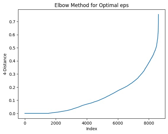
Example visualization created using Elbow Method:

Cluster Detection using DBSCAN:

DBSCAN is one example of a model to create clusters. K-means is also another good alternative.

• The eps parameter controls the maximum distance between two points for them to be considered part of the same neighborhood (i.e., cluster).

• The min_samples parameter determines the minimum number of points required to form a dense region, effectively determining the minimum size of a cluster.

• You can try different values for eps and min_samples based on your dataset.

def detect_clusters_dbscan(embeddings, eps=0.2, min_samples=10):
    dbscan = DBSCAN(eps=eps, min_samples=min_samples, metric='cosine')
    cluster_labels = dbscan.fit_predict(embeddings)
    unique_communities = []
    for label in np.unique(cluster_labels):
        cluster_indices = np.where(cluster_labels == label)[0]
        if len(cluster_indices) >= min_samples:
            unique_communities.append(cluster_indices.tolist())
    return unique_communities

# Call the function
uniques_comm = detect_clusters_dbscan(embeddings, eps=0.3, min_samples=30)

Plot Clusters:

To make it easier to evaluate, we can plot the detected clusters.

def plot_clusters(clusters_to_show):
    NUM_CLUSTERS_TO_USE = len(clusters_to_show)
    print(f"Number of clusters to use: {NUM_CLUSTERS_TO_USE}")
    # if NUM_CLUSTERS_TO_USE > 20:
    #     NUM_CLUSTERS_TO_USE = 20

    sum = 0
    for cluster in clusters_to_show[:NUM_CLUSTERS_TO_USE]:
        sum += len(cluster)

    percentages = []
    for cluster in clusters_to_show:
        percentages.append((len(cluster)/sum)*100.0)

    labels = [f"Cluster{i}" for i in range(1, NUM_CLUSTERS_TO_USE)]
    values = percentages

    fig = go.Figure(data=[go.Pie(labels=labels, values=values, hole=.3)])
    fig.update_layout(width = 720, height = 720)

    return fig

# Call the function
plot_clusters(uniques_comm)

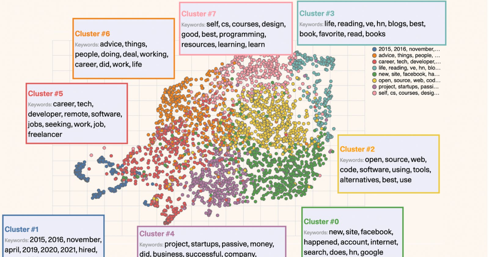
Example visualization created using sample dataset: